Cuckoo Breeding Ground - A Better Cuckoo Hash Table
Abstract
Cuckoo hashing is one of the most popular hashing schemes (theoretically and practically), due to its simplicity, high table load and deterministic worst case access time. However current algorithms are not very memory friendly. Positive lookups (key is in the table) and negative lookups (where it is not) on average access 1.5 and 2.0 buckets (memory regions), respectively, which results in 50 to 100% more memory regions access than should be minimally necessary. This paper introduces a new hash table called Cuckoo Breeding Ground (CBG) based on cuckoo hashing, that access at 90% table load 1.19, 1.09, 1.05 memory regions for negative queries and 1.26, 1.12, 1.07 memory regions for positive queries for windows of size l = 2, 3, 4 respectively. The load threshold is increased to 98.20%, 99.86% and 99.99% for windows of size l = 2, 3, 4 respectively, that compares favorably to 89.70%, 95.91% and 98.04% for the most common blocked-cuckoo. All this with a memory overhead of one byte per element or less and a relatively simple implementation. In many common instances our performance at a table load of 99% is only 15% - 25% worse than theoretically possible, opening new use-cases for a highly memory efficient hash table.
Introduction
A hash table is a data structure that maps items to locations using a hash function. Ideally, the hash function should assign each possible item to a unique location, but this objective is rarely achievable in practice. Two or more items could be mapped to the same location resulting in a collision. A popular way to handle collisions is for the item to have multiple choices for his possible location1. This is sometimes called the power of choice. This lowers the maximum load of a bucket from \(\frac{\log(n)}{\log \log(n)}\) to \(\log \log(n)\) with high probability. Cuckoo hashing2 draws on this idea. Each item is hashed to two locations. If both are used, then the insertion procedure moves previously-inserted items to their alternate location to make space for the new item. The insertion operation in cuckoo hashing is similar to the behavior of cuckoo birds in nature where they kick other eggs/birds out of their nests.
Related Work on Cuckoo Hashing
There are many variants of cuckoo hashing. Here we review the most prominent, but first we define some terms.
- Bin: A memory location where only one element can be stored.
- Bucket: A contiguous collection of bins.
- Table load: The number of elements stored in the hash table divided by the number of bins.
- Load threshold: It is well know the existence of load thresholds in cuckoo hashing. It is a load that can be achieved with high probability but higher loads can not.
Common generalizations
There are three natural ways to generalize cuckoo hashing. The first is to increase the number of hash function used from 2 to a general d ≥ 2. The second is to increase the capacity of a memory location (bucket) k ≥ 2 so that it can store more than one item. This is normally referred as blocked cuckoo and is the most usual option. The third is to have the buckets of size l ≥ 2 overlap. We call this windowed cuckoo and it is explored in 3 and 4. These schemes could of course be combined, hence we define the B(d,k)-cuckoo scheme as one that uses d hash functions and a capacity of k in each bucket. Similarly we can define the W(d,l)-cuckoo scheme as one that uses d hash functions and a window of size l for each bucket. In this terminology the standard cuckoo hashing scheme described previously is the B(2,1)-scheme. The goal of these schemes is to increase the load threshold of the data structure from 50% with vanilla cuckoo hashing.
In practice an increase in d and k or l are not equivalent. Increasing d requires an additional computation of hash function and one more random memory probe which is likely to be a cache miss. On the other hand, a moderate increase in k or l may come with almost no cost at all if the items in the bucket share the same cache line. Thus, an appealing option in practice is setting d = 2 and k = 4 for fast lookup with high table load. When very high table load is needed (>99%), popular configurations are B(2,8) or B(3,8).
Our Contribution
Perhaps the most significant downside of cuckoo hashing, however, is that it potentially requires checking multiple memory regions randomly distributed throughout the table. In many settings, such random access lookups are expensive, making cuckoo hashing a less compelling alternative. We design a variant of cuckoo hashing that reduces the number of memory regions accessed, increase the load threshold and remains relatively simple. We do this by choosing some less popular options for cuckoo hashing with a couple of novel ideas.
Cuckoo Breeding Ground description
Continuing with the bird metaphor, instead of a disjoint set of nests (blocked cuckoo) that is more commonly associated with cuckoo implementations, we view our hash table as one interdependent/intermixing giant and messy breeding ground. We choose the following options:
- Only
d = 2hash functions are used. More affect performance and they are not needed. - One hash function is preferred (called primary) to hash the vast majority of elements so that most lookups only require one bucket access. The other hash function is called secondary.
- Only one table is used instead of the more common
dtables. If we choosed = 2tables, we cannot place more than50%of elements in the primary bucket. - Windowed (overlapping) buckets are used instead of the most common blocked buckets. This provides significantly better table load and more options to mingle the elements.
- Hopscotch5 is used to find an empty bin.
- Anchored Sliding Windows are used instead of only one static window. This harnessed again the power of choice.
- The insertion algorithm used is LSAmax6 with tie-breaking to the primary bucket. The label saved is the minimum of the non-used bucket. This algorithm is based on 7 and 8.
- Unlucky Buckets Trace: We add an additional bit to each bucket representing when any element belonging to this primary bucket were put in a secondary bucket. Note that this is only needed when negative queries are expected, to exclude the check of the secondary bucket.
General Layout
We conceptually use two tables, a metadata table were we store additional information about buckets and items: LSAmax labels, unlucky Buckets trace, buckets orientation plus other details and the other table containing the bins with the elements. Figure 1 show the general layout of our hash table. We call the bin that is selected by the hash function as the entry bin of the bucket and is colored in figure 1.

General layout of CBG
Anchored Sliding Windows
Normally the window used to place and lookup items is static or only oriented forward. We use a window that can dynamically slide around the entry bin (fig 2). It can be easily seen that the number of possible slide positions for the window anchored on the entry bin is l. In this paper we only use two sliding positions: forward and backward (or reverse) (fig 2) because it provides the best tradeoff between benefits/costs. The option to use more sliding positions is leave out for a future research.
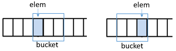
Anchored Sliding Window
Note that adding reverse buckets gives tremendous flexibility to our hash table. For example the last buckets in the table can be fixedly reversed instead of using a more common circular pattern. We can also reverse buckets that cross cache lines to improves performance.
Pseudo code
Below we give a description of the insertion algorithm:
// Insert an item in CBG.
// Return true if it is possible to insert, false otherwise
bool Insert(Item item, Metadata m, HashTable t)
{
  // Get possible locations (buckets) of the items
  Bucket [b_primary, b_secondary] = Get_Locations(item, m);
  // Calculate minimums
  [Bin bin_primary, int min_primary] = Minimum_Label(b_primary, m);
  [Bin bin_secondary, int min_secondary] = Minimum_Label(b_secondary, m);

  // Minimum greater than l_max terminates because
  // more work gives smaller returns
  if (min(min_primary, min_secondary) >= L_MAX)
    return false;

  // Try to insert in the primary bucket
  if(bin_primary.is_empty || Rearrange_Elements(b_primary, m, t, &bin_primary))
  {
    m.labels[bin_primary] = min_secondary + 1;
    t[bin_primary] = item;
    return true;
  }

  // No luck, go secondary
  if(bin_secondary.is_empty || Rearrange_Elements(b_secondary, m, t, &bin_secondary))
  {
    m.labels[bin_secondary] = min_primary + 1;
    m.unlucky_bucket[b_primary] = true;
    t[bin_secondary] = item;
    return true;
  }

  // No empty position found -> cuckoo it
  if(min_primary <= min_secondary)
  {
    m.labels[bin_primary] = min_secondary + 1;

    Item victim = t[bin_primary];
    t[bin_primary] = item;
    return Insert(victim, m, t);
  }
  else
  {
    m.labels[bin_secondary] = min_primary + 1;
    m.unlucky_bucket[b_primary] = true;

    Item victim = t[bin_secondary];
    t[bin_secondary] = item;
    return Insert(victim, m, t);
  }
}
The Rearrange_Elements function try to find an empty bin rearranging the elements. First it try to hopscotch and then try to reverse the bucket. The option to reverse the bucket and then hopscotch in reverse is not tried by the algorithm. It is again a tradeoff decision and future research may explore it.
The other hash table operations are self-explanatory and we do not provide any more discussion on them.
Evaluation (Experiments)
We do a number of experiments to validate our algorithm/model. All random numbers in our simulations are generated by MT19937_64 generator of the standard C++ library. We store the 64-bit generated number as the value in the table. We divide the 64-bit in two halves (secondary_hash = upper and primary_hash = lower) and use them as the two hashes of the element. We repeat the experiment 1000 times and gives the average value. A hash table of 105 bins is used. All code and experimental data can be obtained in this GitHub repository.
Insertion and Lmax
We begin trying to find an adequate value for lmax (table 1). Higher l/lmax values gives higher load threshold and smaller variance. It is noteworthy that the load threshold/variance stabilize when a sufficiently high lmax value is reached. A value of lmax = 7 provides good table load using only 3 bits of additional information. This value is used in all other experiments.
l/lmax | lmax=1 | lmax=2 | lmax=3 | lmax=4 | lmax=5 | lmax=6 | lmax=7 |
|---|---|---|---|---|---|---|---|
l=3 | 27.4% ± 17.1% | 73.4% ± 19.7% | 96.8% ± 5.4% | 99.64% ± 0.64% | 99.82% ± 0.06% | 99.85% ± 0.06% | 99.86% ± 0.05% |
l=4 | 39.8% ± 18.6% | 83.9% ± 12.5% | 99.7% ± 1.3% | 99.98% ± 0.02% | 99.989% ± 0.015% | 99.989% ± 0.015% | 99.990% ± 0.015% |
l=5 | 48.8% ± 20.3% | 90.4% ± 10.6% | 99.98% ± 0.13% | 99.9988% ± 0.010% | 99.9990% ± 0.007% | 99.9990% ± 0.007% | 99.9990% ± 0.007% |
l=6 | 55.8% ± 17.3% | 95.7% ± 9.9% | 99.999% ± 0.031% | 99.9997% ± 0.003% | 99.9998% ± 0.003% | 99.9998% ± 0.003% | 99.9998% ± 0.003% |
Table 1: Comparing different window size l and lmax (cells contain average load threshold with variance)
Load threshold
A very important characteristic of cuckoo hash table is the load threshold. We compare our algorithm to the other common options in table 2 (data taken from 9). Our algorithm is significantly better than the more common blocked cuckoo. With respect to windowed cuckoo we have an advantage of one value of l. Note that for l = 3 our load threshold is similar to windowed l = 4 load threshold. It is apparent that the load threshold will not be an issue with almost any use of our hash table, even when using l = 2.
l/Cuckoo Type | Blocked | Windowed | CBG (our) |
|---|---|---|---|
l=2 | 89.70118682% | 96.4994923% | 98.199973% |
l=3 | 95.91542686% | 99.4422754% | 99.863994% |
l=4 | 98.03697743% | 99.8951593% | 99.990220% |
l=5 | ≈98.96% | ≈99.979018% | 99.999040% |
l=6 | ≈99.41% | ≈99.995689% | 99.999768% |
Table 2: Load threshold for different cuckoos tables/window size
Lookup performance
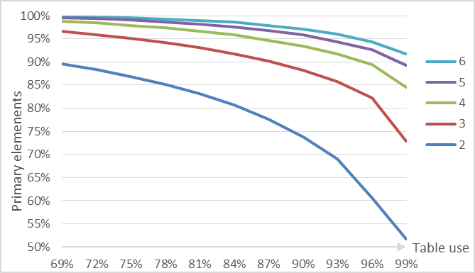
We focus now on the number of memory regions accessed on lookup. We characterize this by two metrics: the number of primary elements (elements that are placed in their primary bucket) and the number of lucky buckets (primary buckets with no element in a secondary bucket). This metrics affect the performance of positive and negative queries respectively. This metrics vary with table load and are similar in value. We show the primary elements metric in figure 3.
Primary elements percent by table load for different values of l
It is clear that the table with l = 2 can not cope well with a modestly high table load, but for l ≥ 3 the picture changes. More interesting is that for very high table load (99%) we have only a performance impact of 25% or 14% for l = 3 and l = 4 respectively (table 3). This means that in many use cases we can have hash tables with almost no wasted space performing only ≈20% worse than optimal.
| Table Load | Param | l=2 | l=3 | l=4 | l=5 | l=6 |
|---|---|---|---|---|---|---|
| 50% | Primary | 95% | 99% | ≈100% | ≈100% | ≈100% |
| Lucky | 98% | ≈100% | ≈100% | ≈100% | ≈100% | |
| Reverse | 2.3% | 1.7% | 1.2% | 0.8% | 0.5% | |
| 75% | Primary | 87% | 95% | 98% | 99% | ≈100% |
| Lucky | 92% | 97% | 99% | 99% | ≈100% | |
| Reverse | 5.0% | 4.8% | 4.3% | 3.6% | 3.1% | |
| 90% | Primary | 74% | 88% | 93% | 96% | 97% |
| Lucky | 81% | 91% | 95% | 97% | 98% | |
| Reverse | 7.1% | 6.9% | 6.5% | 5.9% | 5.4% | |
| 99% | Primary | 52% | 73% | 85% | 89% | 92% |
| Lucky | 60% | 77% | 87% | 90% | 93% | |
| Reverse | 9.1% | 9.0% | 8.5% | 7.9% | 7.2% |
Table 3: Data for different table load/window size.
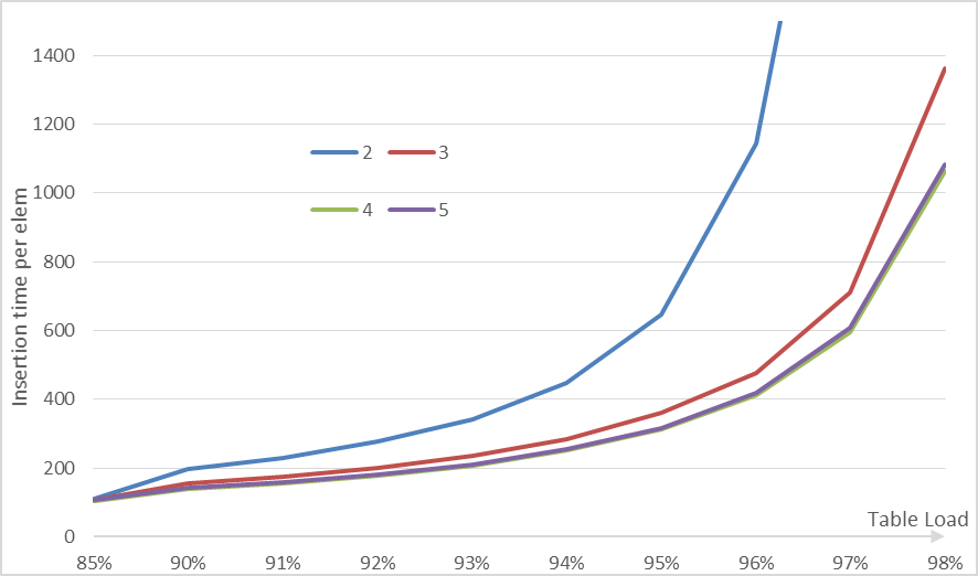
Insertion time
We check the insertion time per element (fig 4). The curve is similar to other cuckoo algorithms. When near the load threshold the insertion time grow exponentially. Note that for all l ≥ 4 the insertion time is practically the same.
For hash tables when the maximum number of items is known, inserting up-to the maximum load is reasonable. But if you do not know this beforehand then it is probably better to grow the table when reaching 94% (or less) by a small grow factor.
Insertion time by table load for different values of l
Metadata overhead
The additional memory our hash table needs to work is important to know. We provide 4 cases (table 4): when the hash table needs to be updated (Read/Write) or not (Read-only) and the majority of query types it will support (negative or positive). For the Item's bucket we provide the value for l = [3, 4] that are the most useful values of l. For l = 2 the value is 2 bits. The Item's bucket is an optimization that removes a hash call when an item is relocated in the same bucket (when hopscotch or reversing the bucket).
| Table Option | Queries | LSAmax label | Item's bucket | Reverse bucket | Unlucky bucket | Total |
|---|---|---|---|---|---|---|
| Read/Write | Negative | 3 bits | 3 bits | 1 bit | 1 bit | 8 bits |
| Positive | 3 bits | 3 bits | 1 bit | 0 bit | 7 bits | |
| Read-only | Negative | 0 bits | 0 bits | 1 bit | 1 bit | 2 bits |
| Positive | 0 bits | 0 bits | 1 bit | 0 bit | 1 bit |
Table 4: Metadata overhead in bits per element.
Note that for l = 4 given the very high table load (99%), small performance hit (15%) and small memory overhead (1 bit) our table may be competitive with Minimal Perfect Hash Tables.
Applicability and the window cost
Until now we do not take into account the cost of overlapping buckets, as some of them may cross into other memory region. When the memory region is significantly larger than the bucket size we may approximate the cost to 0. This happens in many cases:
- Distribute/cloud hash table: Here the memory region is the main memory of each node.
- Magnetic hard disk: Here the main cost is the spinning of the magnetic head, reading consecutive data is fast compared to it.
- TLB cache miss: When accessing memory pages not in the TLB cache. May happen if the hash table is very large.
When the memory region size is in the order of the bucket size we need to take the window cost into our calculation. The most common case here is the CPU cache line that is 64 bytes in mainstream CPUs. We should remark that accessing consecutive cache lines may be cheaper than accessing random cache lines as the hardware prefetcher may kick-in with other optimizations, but this is very difficult to measure and probably processor/architecture specific.
Negative case
We begin our analysis with the negative query case. Adding to the metadata a byte with a fingerprint of each element we have an overhead of 2 bytes per element. Each element have a probability 2/64 = 3.1% of crossing a cache line and a probability 1/256 = 0.4% of a false positive (table 5).
Parameter/l | l=2 | l=3 | l=4 | l=5 | l=6 |
|---|---|---|---|---|---|
| Window Cost | 3.9% | 7.4% | 10.9% | 14.5% | 18.0% |
| load=50% | 1.06 | 1.07 | 1.11 | 1.15 | 1.18 |
| load=75% | 1.12 | 1.10 | 1.12 | 1.16 | 1.18 |
| load=90% | 1.23 | 1.16 | 1.16 | 1.18 | 1.20 |
| load=99% | 1.44 | 1.30 | 1.24 | 1.25 | 1.25 |
Table 5: Cache line cost for negative queries.
The additional cost of windowed cuckoo is small for negative queries but still noticeable. We should note that plain blocked cuckoo negative query average cache line cost is 2.
Positive case
The positive case presents different challenges. We adopt a simple linear layout and test how our table performs under different table loads and element size (table 6).
| Table Load | Element Size | l=2 | l=3 | l=4 | l=5 | l=6 |
|---|---|---|---|---|---|---|
| 50% | 64 bytes | 1.32 | 1.39 | 1.43 | 1.46 | 1.48 |
| 32 bytes | 1.18 | 1.20 | 1.22 | 1.23 | 1.24 | |
| 21 bytes | 1.46 | 1.45 | 1.46 | 1.46 | 1.47 | |
| 16 bytes | 1.12 | 1.10 | 1.11 | 1.12 | 1.12 | |
| 12 bytes | 1.23 | 1.21 | 1.21 | 1.21 | 1.21 | |
| 10 bytes | 1.22 | 1.19 | 1.19 | 1.20 | 1.20 | |
| 9 bytes | 1.22 | 1.19 | 1.19 | 1.19 | 1.19 | |
| 8 bytes | 1.08 | 1.06 | 1.06 | 1.06 | 1.06 | |
| 75% | 64 bytes | 1.59 | 1.75 | 1.89 | 2.01 | 2.09 |
| 32 bytes | 1.36 | 1.40 | 1.46 | 1.51 | 1.55 | |
| 21 bytes | 1.64 | 1.61 | 1.63 | 1.65 | 1.68 | |
| 16 bytes | 1.25 | 1.22 | 1.24 | 1.26 | 1.28 | |
| 12 bytes | 1.36 | 1.31 | 1.31 | 1.32 | 1.33 | |
| 10 bytes | 1.34 | 1.29 | 1.28 | 1.29 | 1.30 | |
| 9 bytes | 1.34 | 1.28 | 1.27 | 1.28 | 1.28 | |
| 8 bytes | 1.19 | 1.14 | 1.13 | 1.13 | 1.14 | |
| 90% | 64 bytes | 1.90 | 2.09 | 2.32 | 2.56 | 2.79 |
| 32 bytes | 1.58 | 1.60 | 1.69 | 1.80 | 1.91 | |
| 21 bytes | 1.87 | 1.79 | 1.81 | 1.87 | 1.93 | |
| 16 bytes | 1.42 | 1.36 | 1.38 | 1.42 | 1.47 | |
| 12 bytes | 1.54 | 1.44 | 1.43 | 1.46 | 1.49 | |
| 10 bytes | 1.52 | 1.41 | 1.40 | 1.41 | 1.43 | |
| 9 bytes | 1.51 | 1.39 | 1.38 | 1.39 | 1.41 | |
| 8 bytes | 1.34 | 1.24 | 1.22 | 1.23 | 1.25 | |
| 99% | 64 bytes | >2.30 | 2.64 | 2.85 | 3.18 | 3.56 |
| 32 bytes | >1.87 | 1.96 | 2.00 | 2.14 | 2.32 | |
| 21 bytes | >2.17 | 2.12 | 2.07 | 2.13 | 2.23 | |
| 16 bytes | >1.65 | 1.61 | 1.58 | 1.62 | 1.70 | |
| 12 bytes | >1.78 | 1.69 | 1.62 | 1.63 | 1.68 | |
| 10 bytes | >1.75 | 1.64 | 1.56 | 1.57 | 1.60 | |
| 9 bytes | >1.74 | 1.62 | 1.54 | 1.54 | 1.57 | |
| 8 bytes | >1.55 | 1.44 | 1.37 | 1.37 | 1.39 |
Table 6: Cache line cost for positive queries.
We should point out that plain blocked cuckoo positive query average cost is 1.5 cache lines IF the bucket is contained completely inside a cache line, so the element size needs to be 16 or 8 bytes. Note that our table can seamless transition from medium elements to larger elements maintaining a good performance.
The first thing to note is that positive query performance is significantly worse than negative query performance. This is because element size is higher than the 2 bytes we use to represent elements in negative queries. Also interesting is that if the element size is not a power of two it may pay to pad each element to a power of two size.
Note that an obvious optimization that is possible in our table is to by default reverse the buckets that are near a cache line end, so the majority of its elements will be inside the cache line. We currently do not do this and may explore the option in the future.
Optimal parameters
It is clear that l = [2, 3, 4] provides the best value with a high enough diversity. Larger l values are very similar in performance to l = 4 and may only be worth it in highly specific conditions.
In general l = 2 can be used with table loads in the range [0% - 50%,70%], l = 3 in [50%,70% - 95%] and l = 4 in [95% - 100%]. If the element size is large (32 bytes or more) and positive queries are the majority, we reduce the l recommendation by one. Note that only one hash table implementation is needed, one that progressively increases l when a specific table load is reached.
If the absolutely best performance is required l = 2 with a table load ≤ 50% is recommended. If no memory can be wasted l = 4 with a table load = 99% is the best option. l = 3 with a table load between 70% and 90% is a more balanced approach.
Conclusions and Future Work
The new hash table Cuckoo Breeding Ground is presented that combines some unpopular cuckoo options with some novel ideas, reducing significantly the number of memory regions access on lookup with an increased load threshold. Our hash table memory overhead is small and the implementation remains relatively simple. Another advantage is increased flexibility and adaptability to varied conditions.
There are many research directions that can be taken from basic CBG. The Anchored Sliding Windows presented in this paper is not fully exploited, so a future research can shed light on how much this idea really helps the overlapping buckets. LSAmax in an overlapping buckets cuckoo hash table may exhibit slightly different properties than in blocked-cuckoo. This needs to be research more thoroughly. We only analyze the online case for insertion. The offline case may be important for Minimal Perfect Hash Tables and other uses. Researching the performance gains obtained by reversing buckets that cross cache lines may proves useful in practical applications. Also using an in-bucket bitmap representing the elements that belong to the bucket may reduce cache lines access.
An observing reader may note that we do not mention the Remove operation. Many hash table use-cases do not need it, but if necessary it may be implemented putting to 0 the removing item bin label. Many Remove operations coupled with Insert operations executed one after the other (maintaining the same table load) generates two problems. The first is that the Unlucky Bucket Trace may degrade over time. Using a counter instead of a bit may solve this problem. The other is that the LSAmax labels of items that reference to the removed item do not decrease, impacting the performance in some ways. This is more complex to solve and probably an in-depth research is needed.
References
- http://epubs.siam.org/doi/abs/10.1137/S0097539795288490 "Yossi Azar, Andrei Z. Broder, Anna R. Karlin, and Eli Upfal. Balanced allocations. SIAM J. Comput., 29(1):180–200, September 1999." ^
- http://dx.doi.org/10.1016/j.jalgor.2003.12.002 "Rasmus Pagh and Flemming Friche Rodler. Cuckoo hashing. J. Algorithms, 51(2):122–144, May 2004" ^
- http://dx.doi.org/10.1007/978-3-642-04128-0_60 "Eric Lehman and Rina Panigrahy. 3.5-way cuckoo hashing for the price of 2-and-a-bit. In Amos Fiat and Peter Sanders, editors, ESA, volume 5757 of Lecture Notes in Computer Science, pages 671–681. Springer, 2009." ^
- http://dx.doi.org/10.1016/j.tcs.2007.02.054 "Martin Dietzfelbinger and Christoph Weidling. Balanced allocation and dictionaries with tightly packed constant size bins. Theoretical Computer Science, 380(1-2):47–68, 2007." ^
- http://mcg.cs.tau.ac.il/papers/disc2008-hopscotch.pdf "Herlihy, Maurice and Shavit, Nir and Tzafrir, Moran. Hopscotch Hashing. Proceedings of the 22nd international symposium on Distributed Computing. Arcachon, France: Springer-Verlag. pp. 350–364. 2008" ^
- research_cuckoo_lsa.md "Alain Espinosa. LSA_max - A Better Insertion for Cuckoo Hashing, 2018" ^
- https://doi.org/10.1007/978-3-642-40450-4_51 "Megha Khosla. Balls into bins made faster. In Algorithms - ESA 2013 - 21st Annual European Symposium, Sophia Antipolis, France, September 2-4, 2013. Proceedings, pages 601–612, 2013" ^
- https://arxiv.org/abs/1611.07786v1 "Megha Khosla and Avishek Anand. A Faster Algorithm for Cuckoo Insertion and Bipartite Matching in Large Graphs. 2016" ^
- http://arxiv.org/abs/1707.06855v2 "Stefan Walzer. Load Thresholds for Cuckoo Hashing with Overlapping Blocks. 2017" ^
Alain Espinosa
Software developer
My research interests include software performance, password security, DSP and ultrasonic communications.