LSA_max - A Better Insertion for Cuckoo Hashing
Abstract
Cuckoo hashing is one of the most popular hashing schemes (theoretically and practically), due to its simplicity, high table load and deterministic worst case access time. However current insertion algorithms have many problems. BFS reach very high table load but it is slow. State-of-the-art Random Walk (RW) is fast but when reaching high table load it degrades strongly. LSA is fast, reaching high table load but is O(n2) in the worst case, needs an additional integer by element and is only defined for (d,1)-schemes. We modify the LSA algorithm for all the schemes (including the more practical (2,k)-schemes) obtaining worst case O(lmaxn) and amortized case O(lmax) for the constant lmax in the range [8 - 2] (more commonly [4 - 2]). We need only an additional [2.5 - 1.1] bits per element. We reach table load similar to BFS and in many cases 2% better than Random Walk. Besides, the algorithm remains simple and can be implemented with high performance in current hardware.
Introduction
A hash table is a data structure that maps items to locations using a hash function. Ideally, the hash function should assign each possible item to a unique location, but this objective is rarely achievable in practice. Two or more items could be mapped to the same location resulting in a collision. A popular way to handle collisions is for the item to had multiple choices for his possible location1. This lowers the maximum load of a bucket from \(\frac{\log(n)}{\log \log(n)}\) to \(\log \log(n)\) with high probability. Cuckoo hashing2 draws on this idea. Each item is hashed to two locations. If both are used, then the insertion procedure moves previously-inserted items to their alternate location to make space for the new item. The insertion operation in cuckoo hashing is similar to the behavior of cuckoo birds in nature where they kick other eggs/birds out of their nests.
There are two natural ways to generalize cuckoo hashing. The first is to increase the number of hash function used from 2 to a general d > 1. The second is to increase the capacity of a memory location (bucket) so that it can store more than one item. We remark that it is also possible to have the buckets overlap. This was shown in 3 to carry some advantages, but henceforth we assume buckets are distinct. These schemes could of course be combined, hence we define the (d,k)-cuckoo scheme as one that uses d hash functions and a capacity of k in each bucket. In this terminology the standard cuckoo hashing scheme described previously is the (2,1)-scheme. The goal of these schemes is to increase the space utilization of the data structure from 50% with vanilla cuckoo hashing.
| d\k | k=1 | k=2 | k=3 | k=4 | k=8 |
|---|---|---|---|---|---|
| d=2 | 50% | 89.7% | 95.9% | 98.0% | 99.8% |
| d=3 | 91.8% | 98.8% | 99.7% | 99.9% | 99.999% |
| d=4 | 97.7% | 99.8% | 99.98% | 99.997% | 99.999% |
Table 1: Load threshold for (d,k)-cuckoo scheme
In practice an increase in d and k are not equivalent. Increasing d requires an additional computation of hash function and one more random memory probe which is likely to be a cache miss. On the other hand, a moderate increase in k may come with almost no cost at all if the items in the bucket share the same cache line. Thus, an appealing option in practice is setting d = 2 and k = 4 for fast lookup with high table load. When very high table load is needed (>99%), popular configurations are (2,8) or (3,8).
Related Work on Insertion Algorithms
One question left unanswered is how to insert an item. In the (2,1)-scheme an item that is kicked-out from its slot has exactly one other potential location, hence the insertion algorithm is self-prescribed. Generally though, an item which was kicked-out may kick-out one of d*k − 1 other items and the insertion algorithm needs to specify which one of those to move. In the following we review some of the options to do that. Clearly in the offline case this is simply a matching problem. We analyze the online case in this paper.
Breadth First Search (BFS)
Consider a bipartite graph where the left side is associated with items and the right side with memory locations. We place an edge (u,b) if b is one of u’s d valid memory locations. Further, if u is placed in b we orient the edge towards u, otherwise it is oriented towards b. An online insertion algorithm can scan this graph starting from u until it finds an empty memory location. A natural algorithm to scan this graph is a BFS, where one of the advantages is that the actual evictions (which presumable are a costly operation) would occur along a shortest path. For (d,1)4 proves that the expected number of memory probes the BFS algorithm performs is some constant exponential in 1/ε.
In 5 they propose and analyze the (2,k)-scheme, under the name blocked-cuckoo-hashing. Similarly, they identify the threshold and show that setting \( k ≥ 1 + \frac{\ln(\frac{1}{ε})}{1 - \ln(2)} \) is sufficient for a space utilization of \(\frac{1}{1 + ε}\). While asymptotically this is similar to that of the (d,1)-scheme, as we mentioned before, in practice an increase in k is less costly than an increase of d. They show that if k is larger, but still \(\mathcal{O}(\ln(\frac{1}{ε}))\) then a BFS insertion algorithm runs in constant time on expectation, again with the constant exponential in \(\frac{1}{ε}\).
In practice a threshold MAX_DEPTH (usually MAX_DEPTH=500) is used to reduce the search space. Even with the threshold this method is expensive to perform for each item.
Random Walk (RW)
The state-of-the-art insertion for cuckoo hashing is the Random Walk algorithm. When an item needs to be kicked-out, a random item out of the d*k items is picked and is moved to a random location out of the remaining d*k − 1 locations. This is tantamount to a random walk on the graph described previously.
In 6, 7 and 8 the algorithm is analyzed. It is shown that the expected insertion time of the Random Walk algorithm is at most log2+δ(d)n where δ(d) → 0 as d increases. The bound hold when d is down all the way to the space utilization threshold. The expected insertion time is constant, but d has to be in the order of \( \frac{\log(\frac{1}{ε})}{ε} \), while recall that the threshold for a space utilization of 1−ε is roughly \(\log(\frac{1}{ε})\). They also show that the maximum insertion time is bounded by logO(1)n.
In practice a threshold MAX_LENGTH_RW (usually MAX_LENGTH_RW=500) is used to guarantee that the algorithm terminates.
Wear Minimization
In 9 they analyze the (d,1)-scheme where d ≥ 3 adding a wear count to each bin. When inserting an item they select the bin with the least wear (breaking ties arbitrarily), and increases the wear of the bin. They show the wear is bound to log log n + O(1) after the insertion of n items into a table of size C*n for a suitable constant C. This constant C appears in practice to be important as they tested relatively small table load (up to only 80%).
MinCounter
In 10 they propose an algorithm that is essentially the same as Wear Minimization, but in the context of a cloud environment. They show experimentally that a counter of 5 bits is enough in practice. They also use relatively small table load (up to 90%).
Local Search Allocation (LSA)
A new algorithm was suggested in 11 called Local Search Allocation, which is also aimed at the (d,1) case. In this algorithm each bin b is given an integer label L(b) initially set to zero (bin is empty). The algorithm proceeds as follow:
bmin ← min L(b1 ,...,bd) : Given an item
xlet b1,...,bd be itsdpossible locations. Find the minimal label among thosedbins (ties broken arbitrarily).L(bmin) ← minj≠min L(bj) + 1 : The label of L(bmin) is updated to be one more than the smallest label of the other
d − 1labels.bmin ← x : The item
xis placed in bin bmin. If there is an item already there it is kicked-out from the bin and reinserted using the same procedure.
The paper proves that if m items could be placed in n bins then no label would ever exceed n−1. This means that the algorithm always finds a placement if one exists and has a worst case running time of O(n2). Further, a label that reaches a value of n is a certificate that no placement exists. Secondly, the paper proves that if the d locations are chosen randomly then with high probability it takes O(n) time to place m items, even as m gets close to the maximum load rate.
There is no known high probability bound on the insertion time for a single item, but experiments reported in 12 suggest the maximum to be logarithmic, and significantly smaller than the maximum of Random Walk algorithm. Further, the total insertion time of items is a full order of magnitude smaller than Random Walk.
The algorithm comes with the additional cost of storing the labels. It is shown that with high probability the labels do not exceed O(log n).
Our Contribution
We create the LSAmax algorithm making a number of modifications to LSA. They reduce the worst case insertion time to O(lmax*n) and the amortized running time to O(lmax) for a very small constant lmax. This maintaining the high table load of BFS and improving the rate compared to Random Walk. We show a way to code the labels to obtain [2.5-1.1] bits per element for different (d,k)-schemes. We show that given the low label size necessary we can speed-up the computation with lookup tables reducing significantly the insertion time.
LSAmax Description
We make three modifications to LSA. First we extend it to arbitrary (d,k)-schemes. The creators of LSA do this in 13, but we consider their choice sub-optimal. Simply consider all the d*k bins as a possible choice for minimum calculation. Clearly some of this positions are not independent of each other (so we lose a lot of the analysis and guarantees) but practical use of cuckoo demonstrate statistics do not change too much. Now all bins had an integer label. In a later section we show that labels inside a bucket are related and how to optimize their memory use.
Second we use a very small constant lmax as the terminating condition. In 14 they note that with a very small maximum number of moves they find an optimal solution for the Delicious dataset, but do not expand on this. We show that the insertion algorithm converges quickly to optimal solutions with respect to lmax, so bigger lmax only gives smaller and smaller returns and therefore are not needed. This permits to stablish a bound on insertion time and reduces the required label size. Intuitively lmax may depend on the maximum number of elements in a given bucket that is log log n (also see 15), so the assumption to be very small is reasonable. In experiments we show lmax a constant depending on the (d,k)-scheme and not n for all practical values of n.
Third we use a tie-breaking strategy for minimum calculation. Given that lmax is very small and we had d*k choices now, a tie-breaking strategy is increasingly important.
Below we give a description of the algorithm:
// Insert an item with LSA_max algorithm.
// Return true if it is possible to insert, false otherwise
bool Insert(Item item, Labels L, HashTable T)
{
  // Get possible locations (buckets) of the items
  Bucket [b_1,...,b_d] = Get_Locations(item, T);
  // Calculate the minimum, 2nd minimum and minimum bin using
  // a tie-breaking strategy
  [Bin bin, int min0, int min1] = Find_Minimums_Labels_Tie_Breaking(L, b_1,...,b_d);

  // Minimum greater than l_max terminates because
  // more work gives smaller returns
  if (min0 >= l_max)
    return false;
  else
  {
    L[bin] = min1 + 1;// update the label with 2nd minimum

    if(bin.Is_Empty())
    {
      T[bin] = item;// save new item
      return true;
    }
    else
    {
      Item kicked_out = T[bin];       // kick-out item
      T[bin] = item;                  // save new item
      return Insert(kicked_out, L, T);// recursively try to insert
    }
  }
}
Analysis
We begin with the following lemma.
Lemma 1: Following the LSAmax algorithm the label of a bin only increase.
Proof (by absurd reduction): suppose Lemma 1 is false →
lorig ≥ l2nd_min+1
lorig > l2nd_min which is false as lorig is selected as the minimum label. □
For the worst case the algorithm visit each occupied bin at most lmax times increasing his label by at least one (by Lemma 1) so the sum of all labels is at worst lmax*n and the algorithm is O(lmax*n). For the amortized version the case is similar and gives O(lmax). Note that the difficult here is not the running time, but if the algorithm can reach high table load and we respond affirmatively in the experiments.
Tie-breaking strategies
We consider three possible strategies for tie-breaking:
- Least loaded: Choose the least loaded of the options. This is the most intuitive option in cuckoo hashing.
- Random: Choose an item randomly.
- Left: Select the item on the left.
For tie-breaking we can consider two cases: inter-bucket or intra-bucket. Option 2 and 3 are self-explanatory for the two cases. For option 1 we define the load of a bucket as the sum of his labels Σi=1,...,k (li). For inter-bucket we choose the least-loaded bucket (as we are comparing buckets) and for intra-bucket we choose the item with the least-loaded alternate bucket (as we are comparing items in the context of a bucket).
Labels coding
Labels in a bucket can be represented with LBsize = k log2 lmax bits in the general case. We can do better considering the relationship of labels inside a bucket. We provide the following lemma:
Lemma 2: *Given a bucket b, lbmax=max_label(b) and lbmin=min_label(b) then lbmax - lbmin ≤ 1*
Proof (by absurd reduction): suppose Lemma 2 is false →
lbmax - lbmin > 1
lbmax > lbmin + 1 → as lbmax is greater than 0 it had an item and was visit before by the algoritm. The last time lbmax was modified lbmax = l2min + 1, substituting
l2min > lbmin by lemma 1 we know that lbmin cannot decrease so when calculating the 2nd minimum the algorithm choose l2min instead of lbmin witch is absurd. □
Joining lemma 1 and lemma 2 we had the following corollary:
Corollary 1: The label of a bin increase at most by 2 at each iteration of LSAmax
By using lemma 2 we can code the labels inside a bucket as the minimum value plus a mask with one bit for each bin specifying the displacement with respect to the minimum. We use LBsize = log2 lmax + k bits for a bucket instead of the LBsize = k log2 lmax in the general case (we can do better noting that the mask with all ones is not a valid state, but we do not consider this in this paper). If we use the intra-bucket tie-breaking strategy Left we can reduce this number further, but it is a complex coding and probably not too flexible (consider removing an item for example). We continue using the more general LBsize = log2 lmax + k on this work.
Evaluation (Experiments)
We do a number of experiments to validate our algorithm/model. All random numbers in our simulations are generated by MT19937_64 generator of the standard C++ library. We store the 64-bit generated number as the value in the table. For d = 2 we divide the 64-bit in two halves (h2 = upper and h1 = lower) and use them as the two hashes of the element. For d > 2 we combine this halves as proposed in 16 to obtain d hashes: hi = h1 + i*h2. We repeat the experiment 1000 times and gives the average value, sometimes mentioned minimum and maximum. We implement cuckoo hashing using only one table instead of the d tables commonly used.
We fist try the tie-breaking strategies for the (2,4)-scheme with 105 bins. Table 2 shows different configurations ordered by table load. Strategy XXX Global means treat all d*k locations as independent applying XXX tie-breaking strategy. LL XXX first resolve inter-bucket ties by Least-Loaded and then apply XXX for intra-bucket ties.
| Strategy/lmax | 1 | 2 | 3 | 4 | 5 | 6 | 7 |
|---|---|---|---|---|---|---|---|
| LL Global | 23.2% ± 11.7% | 95.8% ± 14.4% | 98.0% ± 0.2% | 98.0% ± 0.2% | 98.0% ± 0.2% | 98.0% ± 0.2% | 98.0% ± 0.2% |
| LL LL | 23.0% ± 13.8% | 95.5% ± 3.5% | 98.0% ± 0.2% | 98.0% ± 0.2% | 98.0% ± 0.2% | 98.0% ± 0.2% | 98.0% ± 0.2% |
| LL Left | 49.6% ± 13.2% | 92.4% ± 3.2% | 97.6% ± 0.4% | 98.0% ± 0.2% | 98.0% ± 0.2% | 98.0% ± 0.2% | 98.0% ± 0.2% |
| LL Random | 49.9% ± 14.1% | 91.8% ± 3.4% | 97.5% ± 0.4% | 98.0% ± 0.2% | 98.0% ± 0.2% | 98.0% ± 0.2% | 98.0% ± 0.2% |
| Random Global | 28.6% ± 15.7% | 80.5% ± 15.3% | 96.2% ± 2.8% | 97.9% ± 0.3% | 98.0% ± 0.2% | 98.0% ± 0.2% | 98.0 ± 0.2%% |
| Left Global | 23.1% ± 11.5% | 71.6% ± 18.4% | 93.4% ± 4.6% | 97.5% ± 0.6% | 98.0% ± 0.2% | 98.0% ± 0.2% | 98.0% ± 0.2% |
Table 2: Comparing tie-breaking strategies (cells contain average table load with variance)
The Least-Loaded (LL) strategy provides the fastest convergence; but all converges quickly: at lmax=5 all strategies reach 98% table load. Note that the variance converges to 0.2% quickly too. For lmax=2 the difference between the best and worst strategy is 24%. The difference between the best and random is 15%. Even for lmax=3 the difference between the best and random is 2% with is significant given the high table load. We conclude that a good tie-breaking strategy is important for an optimal convergence.
We are not only interested in table load, but also in other metrics. The average label lavg is one of them. We test different lmax values in Figure 1 with the same (2,4)-scheme with 105 bins.

Comparing average label by tie-breaking strategies
We can see that lavg is similar for similar table load independently of the strategy. Also lavg depends linearly with lmax.
We measure how efficient each strategy are by checking table load at average moves per item. An item is moved when is kicked-out of a position in a bucket. Figure 2 show data for the (2,4)-scheme with 105 bins.
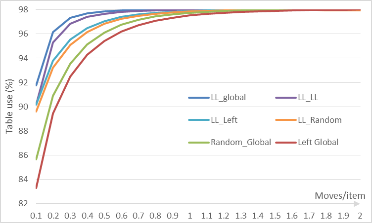
Comparing work done by tie-breaking strategies
Again the Least-Loaded (LL) strategy is the more efficient with LL_Global leading. The results are similar to table 2. We select the strategy LL Left because it have good convergence, is fast to calculate (no need to check alternate locations that may require a hashing done) and may permit better coding of labels to reduce its size. This strategy is used in all the remaining experiments.
We now try common schemes of cuckoo hashing to see how they behaves in figure 3, again with 105 bins.
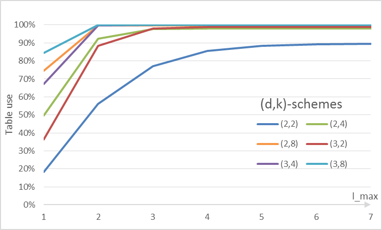
Table load of common cuckoo schemes given lmax
All schemes appear to exhibit similar behavior: a very small constant (<7) lmax when the maximum table load is reached and then increases of lmax do not increases the table load.
The variance (average_value - minimum_value) is similar to table 2, but we perform an additional experiment. We check how table load is distributed again distances to the average value. We repeat the process 10 000 times for the different schemes in figure 4. We use the lmax values of table 3.
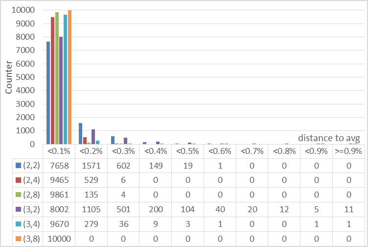
Distribution of table load given distances to the average
From figure 4 it is implied that given a fixed value of d increasing k tighten the distribution around the average. It is a little perplexing that given a fixed k increasing d increases the number near average (<0.1%), but also expand the distribution increasing the numbers away from average (≥0.3%) in (d,k=2,4)-schemes. In any case the errors are minimal: for a distance <0.5% all schemes had probability >99% and many near 100%. This is consistent with the existence of thresholds for random graphs.
From this experiments we can produce the following proposition:
Proposition 1: *For each (d,k)-scheme we can select a very small constant lmax that with high probability results in table load similar to the load threshold. Higher lmax gives infinitesimal small increases in table load.*
We are interested in how much constant lmax really is, as it theoretically may depend on the table size n. We try the (2,4)-scheme with different table sizes in figure 5. It shows that for all practical choices of n (until 1 billion in this test) we can choose a very small lmax (in this case 3 or 4) that is practically independent of n. For example for lmax = 3 the drop in table load was 1% when comparing 102 to 109. With lmax = 4 the drop is only 0.45%. We can expect to handle trillions of elements and continue to consider lmax a constant.

Table load by table size given different lmax
Lookup Tables
Given the small size of labels and the efficient coding of them inside buckets we can consider implementing all label calculation as a table lookup, speeding-up the process significantly. We had d buckets of size LBsize as input and as output a modified bucket label LBsize and d*k positions for the item to be placed. Given this the lookup table size can be calculated as:
LTsize = LBsized * (LBsize + log2 dk)
For the (2,4)-scheme this is 4.5 kb, witch is reasonable. Note that this implementation is incredible fast on practical computers, faster than Random Walk for the selection of the element to be kicked-out. Other efficient implementations without lookup tables are possible given the way we code the labels (using masked comparison on minimum and popcount for Least-Loaded and item selection).
We implement the (2,4)-scheme with a lookup table and compare the performance with Random Walk for different table load in figure 6.
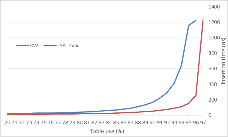
Comparing insertion time for (2,4)-scheme with 105 elements
The insertion time curve is similar to 17 and 18, where LSA is introduced. LSAmax increases the point of inflection of the curve by 5% (note when they both surpass 200 ns) with respect to Random Walk.
For hash tables when the maximum number of items is known, inserting up-to the maximum load is reasonable. But if you do not know this beforehand then it is probably better to grow the table when reaching 94% (in this scheme) by a small grow factor. Note that with high insertion time as provided by LSAmax a small grow is feasible.
Optimal parameters
Given all experiments performed we can now propose optimal parameters for the different schemes in table 3.
| d\k | Parameter | k=2 | k=3 | k=4 | k=8 |
|---|---|---|---|---|---|
| d=2 | Table load (Limit) | 89.7% | 95.9% | 98.0% | 99.8% |
| Table load (RW) | 87.1% | 93.9% | 96.5% | 99.2% | |
| Table load (LSAmax) | 89.7% (lmax=8) | 95.5% (lmax=4) | 98.0% (lmax=4) | 99.6% (lmax=2) | |
| LBsize (bit/elem) | (3+2)/2=2.5 | (2+3)/3=1.7 | (2+4)/4=1.5 | (1+8)/8=1.1 | |
| LTsize | 25x2x(5+2)/8=896 bytes | 25x2x(5+3)/8=1 kb | 26x2x(6+3)/8=4.5 kb | 29x2x(9+4)/8=416 kb | |
| Moves per bin | 1.5 | 0.9 | 1.4 | 0.5 | |
| d=3 | Table load (Limit) | 98.8% | 99.7% | 99.9% | 99.999% |
| Table load (RW) | 97.6% | 99.1% | 99.5% | 99.9% | |
| Table load (LSAmax) | 98.1% (lmax=3) | 99.7% (lmax=3) | 99.7% (lmax=2) | 99.998% (lmax=2) | |
| LBsize (bit/elem) | (2+2)/2=2 | (2+3)/3=1.7 | (1+4)/4=1.25 | (1+8)/8=1.1 | |
| LTsize | 24x3x(4+3)/8=3.5 kb | 25x3x(5+4)/8=36 kb | 25x3x(5+4)/8=36 kb | 29x3x(9+5)/8=224 mb | |
| Moves per bin | 0.6 | 1.1 | 0.5 | 0.7 |
Table 3: Proposed parameters/characteristics of LSAmax for (d,k)-cuckoo scheme
For (d=2,k=2-3-4) LSAmax is 2% more space efficient than Random Walk. For the other configurations is still better but with a low margin. Its table load is similar to BFS. The label size is ≤ 2 bits per element in almost all schemes. The lookup table size LTsize is reasonable for (d=2,k=2-3-4) (d=3,k=2), providing a very fast implementation. The number of items moves (measured by lavg) is small in all cases. The more practical schemes d=2 see the most benefit. Popular (2,4)-scheme is incredible attractive now for a practical implementation with 98% table load, only 1.5 bit per element and lookup table of 4.5kb.
All code and experimental data can be obtained in this GitHub repository.
Conclusions and Future Work
We have presented the new insertion algorithm for cuckoo hashing LSAmax, that can be viewed as a more practical version of LSA. LSAmax extends LSA to all (d,k)-schemes, providing worst case time O(lmax*n) and amortized case O(lmax) for lmax in the range [8 - 2]. It uses a very small bound on label size lmax that together with efficient coding reduces labels size to [2.5 - 1.1] bits per element. The resulting table load is similar to the more expensive BFS and the algorithm can be implemented with high performance.
A theoretical analysis of why lmax is very small remains open, and may provide additional insights on optimization. Also more sophisticated tie-breaking strategies can lead to better performance (For example for the (2,4)-scheme with lmax=3, 10% of item moves are in the same bucket. This may be calculated in advance).
Although experiments with a stash19 do not change results in any significant way, more robust terminating condition may be used. When lmax is reached with still a small table load (bad luck) we can grow lmax, or use a counter of the number of times lmax is reached and use Random Walk here. We remark we do not found this necessary in our experiments.
One possible avenue of work is to optimize for cloud use. Given the low movement of items, LSAmax is a good candidate to a cloud implementation. Substituting Perfect Hash Functions and/or Minimal Perfect Hash Functions for big datasets may also be possible given the low movement of items, fast insertion time, high table load and very low additional memory of labels.
An observing reader may note that we do not mention the Remove operation. Many hash table use-cases do not need it, but if necessary may be implemented putting to 0 the removing item bin label and to 1 the other non-empty bins in the same bucket (this to remain within our lemmas and continue to use the efficient label coding). That this may work within our framework maintaining lmax small is other open research direction to take.
We run all the experiments with the one table implementation, although we do not see any reason not to, it would be nice if the d tables implementation is checked to work similarly under LSAmax.
References
- http://epubs.siam.org/doi/abs/10.1137/S0097539795288490 "Yossi Azar, Andrei Z. Broder, Anna R. Karlin, and Eli Upfal. Balanced allocations. SIAM J. Comput., 29(1):180–200, September 1999." ^
- http://dx.doi.org/10.1016/j.jalgor.2003.12.002 "Rasmus Pagh and Flemming Friche Rodler. Cuckoo hashing. J. Algorithms, 51(2):122–144, May 2004" ^
- http://dx.doi.org/10.1007/978-3-642-04128-0_60 "Eric Lehman and Rina Panigrahy. 3.5-way cuckoo hashing for the price of 2-and-a-bit. In Amos Fiat and Peter Sanders, editors, ESA, volume 5757 of Lecture Notes in Computer Science, pages 671–681. Springer, 2009." ^
- http://dx.doi.org/10.1007/s00224-004-1195-x "Dimitris Fotakis, Rasmus Pagh, Peter Sanders, and Paul G. Spirakis. Space efficient hash tables with worst case constant access time. Theory Comput. Syst., 38(2):229–248, 2005." ^
- http://dx.doi.org/10.1016/j.tcs.2007.02.054 "Martin Dietzfelbinger and Christoph Weidling. Balanced allocation and dictionaries with tightly packed constant size bins. Theoretical Computer Science, 380(1-2):47–68, 2007." ^
- https://arxiv.org/abs/1006.1231 "Nikolaos Fountoulakis, Konstantinos Panagiotou, and Angelika Steger. On the insertion time of cuckoo hashing. SIAM J. Comput., 42(6):2156–2181, 2013." ^
- http://dx.doi.org/10.1137/090770928 "Alan Frieze, Páll Melsted, and Michael Mitzenmacher. An analysis of random-walk cuckoo hashing. SIAM J. Comput., 40(2):291–308, March 2011." ^
- https://arxiv.org/abs/1602.04652v9 "Alan M. Frieze and Tony Johansson. On the insertion time of random walk cuckoo hashing. CoRR, abs/1602.04652, 2016." ^
- https://arxiv.org/abs/1404.0286v1 "David Eppstein, Michael T. Goodrich, Michael Mitzenmacher, and Paweł Pszona. Wear Minimization for Cuckoo Hashing: How Not to Throw a Lot of Eggs into One Basket. 2014" ^
- http://ieeexplore.ieee.org/abstract/document/7208292/ "Yuanyuan Sun, Yu Hua, Dan Feng, Ling Yang, Pengfei Zuo, Shunde Cao. MinCounter: An Efficient Cuckoo Hashing Scheme for Cloud Storage Systems. 2015" ^
- https://doi.org/10.1007/978-3-642-40450-4_51 "Megha Khosla. Balls into bins made faster. In Algorithms - ESA 2013 - 21st Annual European Symposium, Sophia Antipolis, France, September 2-4, 2013. Proceedings, pages 601–612, 2013" ^
- https://doi.org/10.1007/978-3-642-40450-4_51 "Megha Khosla. Balls into bins made faster. In Algorithms - ESA 2013 - 21st Annual European Symposium, Sophia Antipolis, France, September 2-4, 2013. Proceedings, pages 601–612, 2013" ^
- https://arxiv.org/abs/1611.07786v1 "Megha Khosla and Avishek Anand. A Faster Algorithm for Cuckoo Insertion and Bipartite Matching in Large Graphs. 2016" ^
- https://arxiv.org/abs/1611.07786v1 "Megha Khosla and Avishek Anand. A Faster Algorithm for Cuckoo Insertion and Bipartite Matching in Large Graphs. 2016" ^
- https://arxiv.org/abs/1404.0286v1 "David Eppstein, Michael T. Goodrich, Michael Mitzenmacher, and Paweł Pszona. Wear Minimization for Cuckoo Hashing: How Not to Throw a Lot of Eggs into One Basket. 2014" ^
- ftp://ftp.deas.harvard.edu/techreports/tr-02-05.pdf "Adam Kirsch and Michael Mitzenmacher. Less hashing, same performance: Building a better bloom filter. In Yossi Azar and Thomas Erlebach, editors, 14th European Symposium on Algorithms (ESA), number 4168 in LNCS, pages 456–467. Springer, 2006" ^
- https://doi.org/10.1007/978-3-642-40450-4_51 "Megha Khosla. Balls into bins made faster. In Algorithms - ESA 2013 - 21st Annual European Symposium, Sophia Antipolis, France, September 2-4, 2013. Proceedings, pages 601–612, 2013" ^
- https://arxiv.org/abs/1611.07786v1 "Megha Khosla and Avishek Anand. A Faster Algorithm for Cuckoo Insertion and Bipartite Matching in Large Graphs. 2016" ^
- http://epubs.siam.org/doi/abs/10.1137/080728743 "A. Kirsch, M. Mitzenmacher, and U Wieder. More robust hashing: Cuckoo hashing with a stash. SIAM Journal on Computing, vol. 39, no. 4, pp. 1543-1561, 2009." ^
Alain Espinosa
Software developer
My research interests include software performance, password security, DSP and ultrasonic communications.